


Relational databases are powerful tools for analyzing and manipulating data. However, many modeling workflows require a great deal of time and effort to wrangle data from databases to place it into a flat data frame or table format. Only then the actual data analysis can start.
 Photo by Jordan McDonald
Why a relational model?
With the proper tools, analysis can begin using a relational model that works directly with the database. And, if wrangling is still required, R users can leverage this powerful and proven SQL approach to data organization and manipulation.
The dm package takes the primary advantage of databases – relational modeling – and brings it to R. In relational databases, tables or data frames link through primary keys (PK) and foreign keys (FK). Instead of having a single, wide table to work with, data is segmented across multiple tables to eliminate or reduce redundancies. This process is called normalization. A classic example is storing unique identifiers in a large table and looking up values for these unique identifiers in a small data frame. This approach lets an analysis run without reading or writing look-up values until necessary because unique identifiers are enough for most of the runtime.
dm 0.1.1 is available on CRAN. You can now download and install dm, from CRAN, with the following command:
install.packages("dm")
Connect to a database
We connect to a relational dataset
repository with a database server that
is publicly accessible without registration. There is a financial
dataset that contains
loan data, along with relevant information and transactions. We chose
this loan dataset because the relationships between loan, account,
and transcactions tables are good representations of databases that
record real-world business transactions.
The dataset page lists the credentials required for connecting to the database:
- hostname: relational.fit.cvut.cz
- port: 3306
- username:
guest - password:
relational - database:
Financial_ijs
These can be used, for example, in MySQL Workbench to download the CSV data manually. To automate and keep the data in the database for as long as possible, we can connect to the database from R through its database interface to access the tables:
library(RMariaDB)
my_db <- dbConnect(
  MariaDB(),
  user = 'guest',
  password = 'relational',
  dbname = 'Financial_ijs',
  host = 'relational.fit.cvut.cz'
)
dbListTables(my_db)

## [1] "accounts"  "cards"     "clients"   "disps"     "districts" "loans"
## [7] "orders"    "tkeys"     "trans"
By creating a dm object from the connection, we get access to all tables:
library(dm)
my_dm <- dm_from_src(my_db)

my_dm

## ── Table source ────────────────────────────────────────────────────────────────
## src:  mysql  [guest@relational.fit.cvut.cz:NA/Financial_ijs]
## ── Metadata ────────────────────────────────────────────────────────────────────
## Tables: `accounts`, `cards`, `clients`, `disps`, `districts`, … (9 total)
## Columns: 57
## Primary keys: 0
## Foreign keys: 0
names(my_dm)

## [1] "accounts"  "cards"     "clients"   "disps"     "districts" "loans"
## [7] "orders"    "tkeys"     "trans"
my_dm$accounts

## # Source:   table<accounts> [?? x 4]
## # Database: mysql [guest@relational.fit.cvut.cz:NA/Financial_ijs]
##      id district_id frequency        date
##   <int>       <int> <chr>            <date>
## 1     1          18 POPLATEK MESICNE 1995-03-24
## 2     2           1 POPLATEK MESICNE 1993-02-26
## 3     3           5 POPLATEK MESICNE 1997-07-07
## 4     4          12 POPLATEK MESICNE 1996-02-21
## 5     5          15 POPLATEK MESICNE 1997-05-30
## 6     6          51 POPLATEK MESICNE 1994-09-27
## # … with more rows
The components of this particular dm object are lazy tables powered by dbplyr. This package translates the dplyr grammar of data manipulation into queries the database server understands. The advantage to a lazy table is that there is no data download until results are collected for printing or local processing. Below, the summary operation is computed on the database, and only the results are sent back to the R session.
library(dplyr)
my_dm$accounts %>%
  group_by(district_id) %>%
  summarize(n = n()) %>%
  ungroup()

## # Source:   lazy query [?? x 2]
## # Database: mysql [guest@relational.fit.cvut.cz:NA/Financial_ijs]
##   district_id n
##         <int> <int64>
## 1           1 554
## 2           2  42
## 3           3  50
## 4           4  48
## 5           5  65
## 6           6  48
## # … with more rows
If the data fits into your RAM, a database connection is not required
to use dm. The collect() command downloads all tables for our dm
object.
my_local_dm <-
  my_dm %>%
  collect()

object.size(my_local_dm)
## 77922024 bytes
my_local_dm$accounts %>%
  group_by(district_id) %>%
  summarize(n = n()) %>%
  ungroup()

## # A tibble: 77 x 2
##   district_id     n
##         <int> <int>
## 1           1   554
## 2           2    42
## 3           3    50
## 4           4    48
## 5           5    65
## 6           6    48
## # … with 71 more rows
A dm object can also be created from individual data frames with the
dm() function.
Define primary and foreign keys
Relational database tables link to each other via primary and foreign keys. The model diagram provided by our test database illustrates the intended relationships.
However, it turns out this is not an accurate representation of the entities and relationships within the database:
- Table names in our database have the plural form; in the diagram it’s singular.
- There is a
tkeystable available in the database that is not listed in the model diagram. - The
Financial_stddatabase is similar, but different from the one that we work with,Financial_ijs.
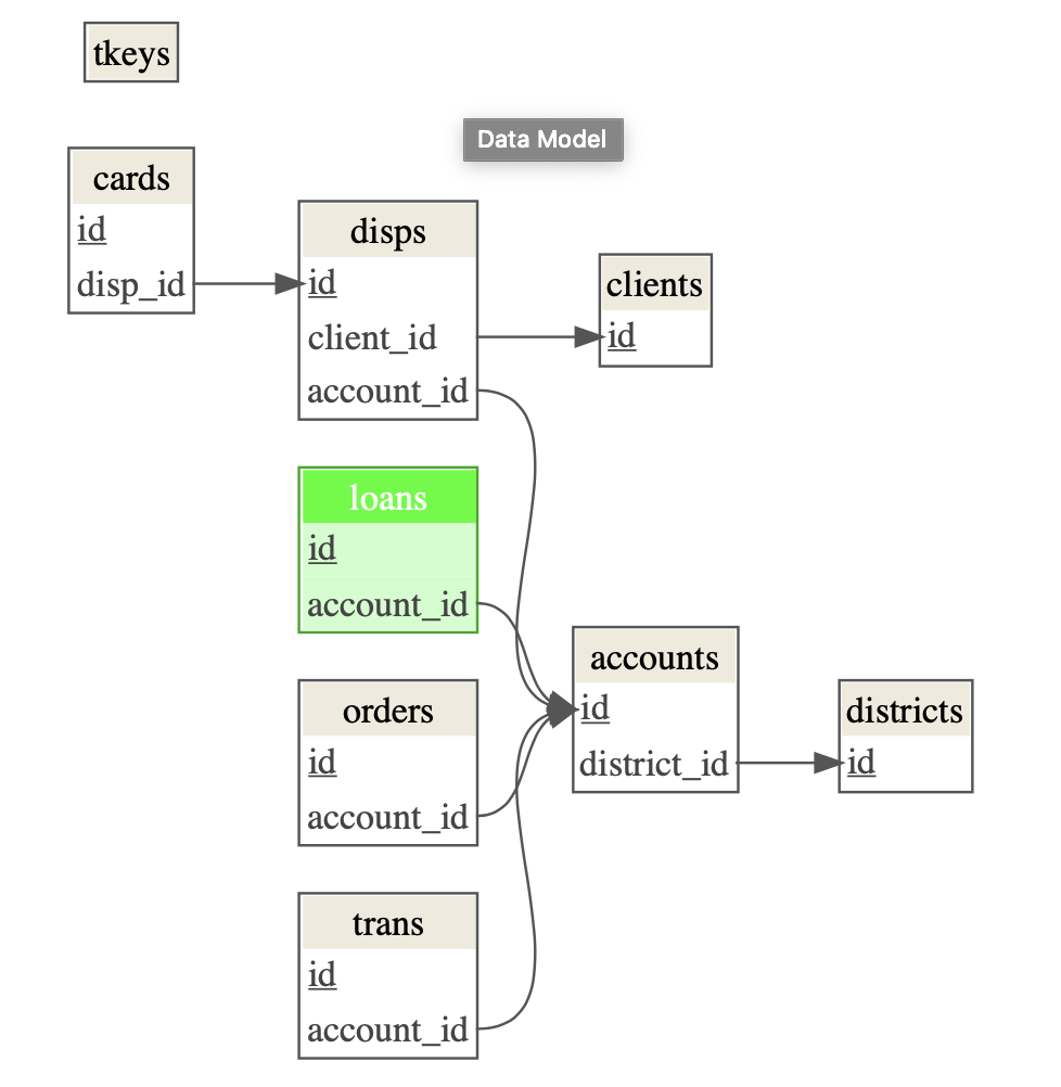
Bearing these discrepancies in mind, we can define suitable primary and
foreign keys for our dm object. The documentation suggests that the
loans table is the most important one. We color the target table
separately with dm_color().
# Defining PKs and FKs
my_dm_keys <-
  my_local_dm %>%
  dm_add_pk(districts, id) %>%
  dm_add_pk(accounts, id) %>%
  dm_add_pk(clients, id) %>%
  dm_add_pk(loans, id) %>%
  dm_add_pk(orders, id) %>%
  dm_add_pk(trans, id) %>%
  dm_add_pk(disps, id) %>%
  dm_add_pk(cards, id) %>%
  dm_add_fk(loans, account_id, accounts) %>%
  dm_add_fk(orders, account_id, accounts) %>%
  dm_add_fk(trans, account_id, accounts) %>%
  dm_add_fk(disps, account_id, accounts) %>%
  dm_add_fk(disps, client_id, clients) %>%
  dm_add_fk(accounts, district_id, districts) %>%
  dm_add_fk(cards, disp_id, disps) %>%
  dm_set_colors(green = loans)

# Draw the visual model
my_dm_keys %>%
  dm_draw()
The discrepancies highlight the importance of being able to define primary and foreign keys. Most of the challenges in manipulating data are not syntax knowledge gaps. The syntax can always be looked up with search engines. Knowledge gaps regarding how data is organized are much more common as stumbling blocks for R users when working with distributed data.
Insight into the structure of a database using the built-in dm_draw()
function provides an instant efficiency boost. Combined with defining
unique identifiers (primary keys) and how they are found by other tables
(foreign keys), an R user can quickly clarify the structures with which
they are working.
To assist with this process of defining the structure, dm comes with a built-in helper to check the referential integrity of the dataset:
my_dm_keys %>%
  dm_examine_constraints()

## ℹ All constraints satisfied.
Create a dataset ready for analysis
For modeling, a flat table or matrix is required as input. If normalization is the process of splitting up a table to reduce redundancies, joining multiple tables together is called denormalizing.
The dm_squash_to_tbl() function creates a denormalized table by
performing a cascading join between cards and all outgoing foreign
keys. A join is the SQL term for combining some or all of the unique
columns between 2 or more tables into a single table using the
appropriate keys. In this case, the cards table has a foreign key to
disps table, which has a foreign key to accounts, which also has a
foreign key to the districts table. These foreign key relationships
are then used in a cascading join within the dm_squash_to_tbl()
function, without having to specify the relationships because they are
already encoded within the dm object.
my_dm_keys %>%
  dm_squash_to_tbl(cards)

## Renamed columns:
## * type -> cards$cards.type, disps$disps.type
## * district_id -> accounts$accounts.district_id, clients$clients.district_id

## # A tibble: 892 x 28
##      id disp_id cards.type issued     client_id account_id disps.type
##   <int>   <int> <chr>      <date>         <int>      <int> <chr>
## 1     1       9 gold       1998-10-16         9          7 OWNER
## 2     2      19 classic    1998-03-13        19         14 OWNER
## 3     3      41 gold       1995-09-03        41         33 OWNER
## 4     4      42 classic    1998-11-26        42         34 OWNER
## 5     5      51 junior     1995-04-24        51         43 OWNER
## 6     7      56 classic    1998-06-11        56         48 OWNER
## # … with 886 more rows, and 21 more variables: accounts.district_id <int>,
## #   frequency <chr>, date <date>, A2 <chr>, A3 <chr>, A4 <int>, A5 <int>,
## #   A6 <int>, A7 <int>, A8 <int>, A9 <int>, A10 <dbl>, A11 <int>, A12 <dbl>,
## #   A13 <dbl>, A14 <int>, A15 <int>, A16 <int>, birth_number <chr>,
## #   clients.district_id <int>, tkey_id <int>
We have an analysis-ready dataset available to use!
Transform data in a dm
Data transformation in dm is done by zooming on the table with which you would like to work. A zoomed dm supports dplyr operations on the zoomed table: simple transformations, grouped operations, joins, and more.
my_dm_keys %>%
  dm_zoom_to(accounts) %>%
  group_by(district_id) %>%
  summarize(n = n()) %>%
  ungroup() %>%
  left_join(districts)

## # Zoomed table: accounts
## # A tibble:     77 x 17
##   district_id     n A2    A3        A4    A5    A6    A7    A8    A9   A10   A11
##         <int> <int> <chr> <chr>  <int> <int> <int> <int> <int> <int> <dbl> <int>
## 1           1   554 Hl.m… Prag… 1.20e6     0     0     0     1     1   100 12541
## 2           2    42 Bene… cent… 8.89e4    80    26     6     2     5    47  8507
## 3           3    50 Bero… cent… 7.52e4    55    26     4     1     5    42  8980
## 4           4    48 Klad… cent… 1.50e5    63    29     6     2     6    67  9753
## 5           5    65 Kolin cent… 9.56e4    65    30     4     1     6    51  9307
## 6           6    48 Kutn… cent… 7.80e4    60    23     4     2     4    52  8546
## # … with 71 more rows, and 5 more variables: A12 <dbl>, A13 <dbl>, A14 <int>,
## #   A15 <int>, A16 <int>
The columns used by left_join() to consolidate tables are inferred
from the primary and foreign keys already encoded within the dm
object.
Reproducible dataflows with dm
Walking through dm’s data modeling fundamentals, adding keys, and drawing the structure, will help R users better understand data from external databases or apply best practices from relational data modeling to their local data.
You can immediately start testing on an Rstudio cloud instance! For more examples and explanations, check out the documentation page. Install this package today!