


Not having a time series at the desired frequency is a common problem for researchers and analysts. For example, instead of quarterly sales, they only have annual sales. Instead of a daily stock market index, they only have a weekly index. While there is no way to fully make up for the missing data, there are useful workarounds: with the help of one or more high-frequency indicator series, the low-frequency series may be disaggregated into a high-frequency series.
 Photo by Jordan McDonald
The package tempdisagg implements the standard methods for temporal disaggregation: Denton, Denton-Cholette, Chow-Lin, Fernandez and Litterman. Our article on temporal disaggregation of time series in the R-Journal describes the package and the theory of temporal disaggregation in more detail.
The package has been around for eight years, enabling the standard year
or quarter to month or quarter disaggregation. With version 1.0, there
are now some major new features: disaggregation can be performed from
any frequency to any frequency. Also, tempdisagg now supports time
series classes other than ts.
Convert between any frequency
tempdisagg can now convert between most frequencies, for example, it can disaggregate a monthly series to daily. It is no longer restricted to regular conversions, where each low-frequency period had the same number of high-frequency periods. Instead, a low-frequency period (e.g. month) can contain any number of high-frequency periods (e.g. 31, 28 or 29 days). Thanks to Roger Kissling and Stella Sim who have suggested this idea.
We can not only convert months to days, but also years to days, weeks to seconds, or academic years to seconds, or lunar years to hours,etc. The downside is that the computation time depends on the number of observations. Thus, for longer high-frequency series, the computation may take a while.
In the following, we try to disaggregate quarterly GDP of Switzerland to a hypothetical daily GDP series. The example series are shipped with the package.
library(tempdisagg)
data(tempdisagg)
head(gdp.q)
##         time    value
## 1 2005-01-01 133101.3
## 2 2005-04-01 136320.4
## 3 2005-07-01 137693.7
## 4 2005-10-01 139475.9
## 5 2006-01-01 139204.7
## 6 2006-04-01 141112.5
Time series can be stored in data frames
Because we are dealing with daily data, we keep the data in a
data.frame, rather than in a ts object. Other time series objects,
such as xts and tsibble, are possible as well. For conversion and
visualization, we use the tsbox package.
library(tsbox)
ts_plot(gdp.q, title = "Swiss GDP", subtitle = "real, not seasonally adjusted")
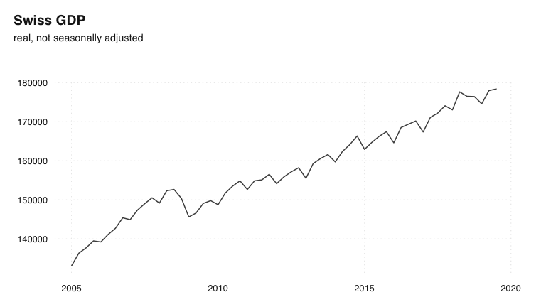 Series to disaggregate: quarterly gross domestic product of Switzerland
Disaggregation to daily frequency
While disaggregation can also be performed without other series, we use
Swiss stock market data as an indicator series to disaggregate GDP. Data
of the stock market index, the SMI, is also included in tempdisagg.
Weekend and holiday values have been interpolated, because td does not
allow the presence of missing values.
ts_plot(spi.d, title = "Swiss Performance Index", subtitle = "daily values, interpolated")
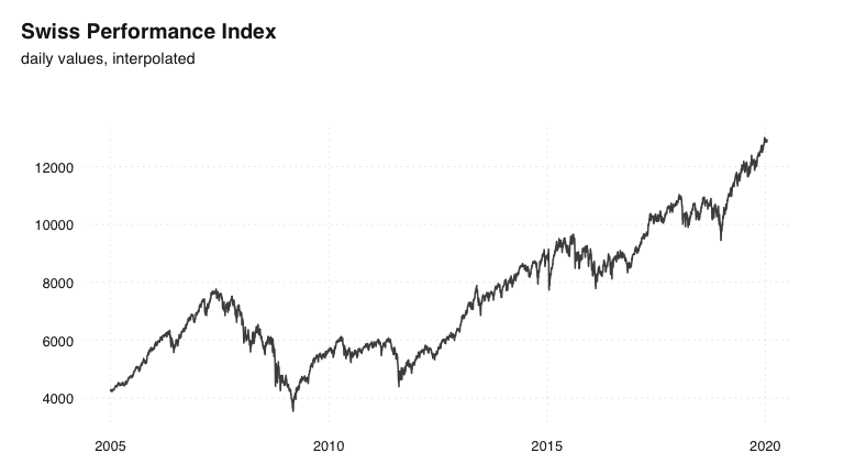 Daily indicator series: Swiss Performance Index
The following uses the Chow-Lin method to disaggregate the series. A high rho parameter takes into account that the two series are unlikely to be co-integrated.
m.d.stocks <- td(gdp.q ~ spi.d, method = "chow-lin-fixed", fixed.rho = 0.9)
summary(m.d.stocks)
##
## Call:
## td(formula = gdp.q ~ spi.d, method = "chow-lin-fixed", fixed.rho = 0.9)
##
## Residuals:
##    Min     1Q Median     3Q    Max
## -10656  -1760   1076   3796   8891
##
## Coefficients:
##              Estimate Std. Error t value Pr(>|t|)
## (Intercept) 1.320e+03  2.856e+01   46.22   <2e-16 ***
## spi.d       5.512e-02  3.735e-03   14.76   <2e-16 ***
## ---
## Signif. codes:  0 '***' 0.001 '**' 0.01 '*' 0.05 '.' 0.1 ' ' 1
##
## 'chow-lin-fixed' disaggregation with 'sum' conversion
## 59 low-freq. obs. converted to 5493 high-freq. obs.
## Adjusted R-squared: 0.7928 AR1-Parameter:   0.9
And here is the result: A daily series of GDP
gdp.d.stocks <- predict(m.d.stocks)
ts_plot(
  ts_scale(
    ts_c(gdp.d.stocks, gdp.q)
  ),
  title = "Daily disaggregated GDP",
  subtitle = "one indicator"
)
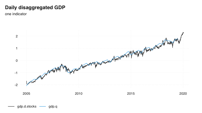 Swiss GDP, disaggregated to daily
Like with all disaggregation methods in tempdisagg, the resulting series fulfills the aggregation constraint (the resulting series is as long as the indicator, and needs to be shortened for a comparison):
all.equal(
  ts_span(
    ts_frequency(gdp.d.stocks, "quarter", aggregate = "sum"),
    end = "2019-07-01"
  ),
  gdp.q
)
## [1] TRUE